Build an LSTM Neural Network Bot for Trading

At the moment’s Mannequin

Full GitHub Link

Hey there everybody. My title’s Aditya, a developer advocate right here at Blankly.

At the moment, we’ll take a look at utilizing the Blankly bundle to construct a primary machine studying mannequin for buying and selling. Machine studying has been one of many hottest developments in algotrading throughout the previous few years, as we have solely just lately reached the extent of computing energy and quantity of knowledge wanted to construct and practice profitable fashions. This particular mannequin we can be an LSTM (Long Short Term Memory) Neural Network, which is a sort of neural community that shops a “reminiscence”, permitting it to include previous knowledge handed into the mannequin into future predictions. This construction makes LSTMs nice for sequential knowledge, like inventory costs.

To construct the mannequin, we’ll use PyTorch, a well-liked library for Machine Studying. Fortunately, PyTorch handles many of the exhausting work for us — backpropagation, gradient descent, and layer construction, to call a number of examples — so we will concentrate on constructing the precise mannequin.

LSTMs

The primary query you might need is what’s an LSTM? As we mentioned above, LSTMs incorporate a “reminiscence” into their mannequin construction, however that rationalization is a bit obscure. To be extra exact, LSTMs compute a number of features at each stage:

With out getting too technical, $h_t$ is the “hidden state” — the “reminiscence” of the mannequin, $f_t$ is the “overlook gate”, $i_t$ is the “enter gate”, $o_t$ is the output gate, $tilde{C}_t$ is the candidate cell state, and $C_t$ is the cell state. At each step, the enter to the mannequin will get handed into the enter gate, influences the hidden state, and doubtlessly modified the cell state. The choices for a way every enter impacts the remainder of the mannequin are determined by neural community layers, that are the weights we practice utilizing gradient descent.

For his or her capacity to dynamically embrace knowledge prior to now in present fashions, LSTMs are one of the vital standard fashions for inventory prediction. There are numerous technical indicators for monetary markets, and so utilizing LSTMs permits us to dynamically select which knowledge from which era body is most related to predicting future costs.

Stock Market Predictions with LSTM in Python – DataCamp

Machine Learning to Predict Stock Prices – Data Science

Using Keras LSTM Model to Predict Stock Prices – KDNuggets

Issues to Watch Out For

There are undoubtedly pitfalls to assuming LSTMs robotically result in success. For one, prediction accuracy is proscribed by the accessible coaching knowledge, and our coaching set is pretty restricted and primary. Nevertheless, usually, short-term inventory value knowledge has a component of randomness, so the accuracy of LSTM predictions has is proscribed. Because of this, we’ll use a median of three predictions — on this means, we’ll cut back inaccuracy as a consequence of randomness, and so enhance total outcomes.

Overview

First, we’ll initialize all the weather of the environment — the keys for the API we want, in addition to the imported libraries we want. Then, we’ll course of the enter knowledge we’ve got and convert right into a format that’s acceptable for mannequin coaching. Then, we’ll run via our coaching loop and discover the optimum weights for our mannequin. After that, we’ll discover a option to convert output indicators from our mannequin into choices onto whether or not to purchase and promote, together with how a lot, and use these to outline a method. Lastly, we’ll backtest this technique and analyze its efficiency to find out whether or not to make use of it for dwell crypto buying and selling or to enhance it additional.

Initialization

We’ll initialize the fundamentals of our Blankly setting with the command blankly init. As soon as executed, we get template .json information that we’ll want for configuring backtests. Most significantly, we’ll have to enter our API keys into keys.json.

$ blankly init

Listed below are our imports. We’ll import blankly (after all), NumPy to be used with getting ready our knowledge, and a few PyTorch utilities we’ll want for our mannequin

import numpy as np
import torch
import torch.nn as nn
import torch.nn.purposeful as F
from torch.nn import LSTM
import torch.optim as optim
from torch.autograd import Variable

Information Preparation

This technique will assist us break up the info into “enter/output”. We solely even have one sequence of knowledge — all the costs from the previous 12 months. Nevertheless, we will generate smaller “episodes” by

1. Taking all consecutive intervals of size seq_length
2. Splitting off the final output_size values and placing these into one array
3. Leaving the primary seq_length – output_size values into one other array.

Ultimately, we’re left with sufficient knowledge to run coaching on. For this mannequin, we’ll use seq_length = 8 and output_size = 3, however these are considerably arbitrary. This provides us coaching sequences of 8 – 3 = 5 knowledge factors to foretell the sequences of size 3 from. The concept is that we’ll practice the mannequin on these sequences of 5 knowledge factors, find yourself with a mannequin that may predict the value actions for the following 3 days to strong accuracy, after which common the value actions over a 3-day interval to acquire a closing prediction for the value motion on a day. Then, we’ll use our prediction to determine whether or not to purchase our promote — if our mannequin tells us the value is prone to improve tomorrow, we’ll purchase, and if the mannequin tells us the value is prone to lower, we’ll promote.

def  episode_gen(knowledge, seq_length,output_size):
    x = []
    y = []
    #Loop via knowledge, including enter knowledge to x array and output knowledge to y array
    for i in  vary(len(knowledge)-seq_length):
        _x = knowledge[i:(i+seq_length - output_size)]
        _y = knowledge[i+seq_length - output_size:i + seq_length]
        x.append(_x)
        y.append(_y)

    return np.array(x),np.array(y)

Mannequin Inputs and Characteristic Engineering

Right here, we’ll do nearly all of work on our mannequin.

To begin, we’ll pull the info we want. Blankly comes with in-built indicators, so we will enter our historic value knowledge into these features to get indicators out. For this instance, we’ll use RSI and MACD. RSI stands for Relative Power Index, and is a measure of momentum. Its system is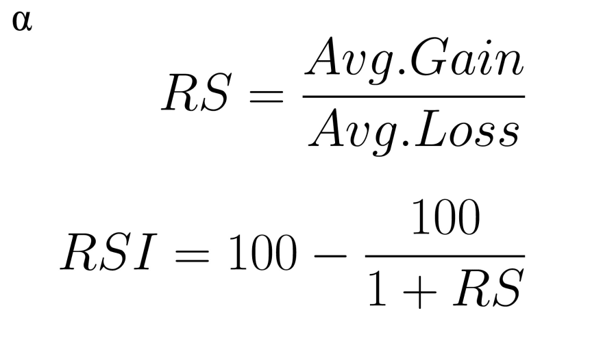

the place we take a look at the info over the previous 14 days. Typical overbought/oversold ranges for RSI are 70 and 30 (respectively)

MACD stands for Shifting Common Convergence Divergence. The MACD is calculated by subtracting the 26-period exponential shifting common (EMA) from the 12-period EMA. We then calculate the MACD sign line by taking the 9-period EMA of the MACD.

Implementing these features by hand is a bit tough, however luckily, Blankly has indicators in-built.

def init_NN(image, state: blankly.StrategyState):

    interface = state.interface
    decision = state.decision
    variables = state.variables

# Get value knowledge

    variables['history'] = interface.historical past(image, 300, decision, return_as='record')['close']

'''We use Blankly's built-in indicator features to calculate indicators we will use together with value knowledge to foretell future costs
'''
    rsi = blankly.indicators.rsi(state.variables['history'])
    macd = blankly.indicators.macd(state.variables['history'])

'''We'll break the historic Ethereum knowledge into 8 day episodes

and try to predict the ultimate three days utilizing the primary 5.

'''
    seq_length = 8
    output_size = 3

We additionally do a little bit of function engineering. Step one is to transform our value knowledge into every day will increase by dividing every day’s value knowledge by the day earlier than. This helps in coaching by “scaling” the info into the identical vary. We’ll additionally restrict the vary of knowledge to the vary during which we’ve got knowledge on all indicators — day 26 and on.

'''Characteristic engineering -- right here, we calculate the value change from the day earlier than
as a ratio. That is helpful as a result of it means we've got much less points with scaling with the mannequin,
as the info will all already be in roughly the identical vary. We ignore the primary 25 components
as a result of we would like each remark to have corresponding RSI + MACD knowledge, and MACD requires
26 intervals.
'''

    x = [variables['history'][i] / variables['history'][i-1] for i in  vary(25,len(variables['history']))]
    x, y = episode_gen(x, seq_length, output_size)
    y = Variable(torch.Tensor(np.array(y))).unsqueeze(0)

#RSI knowledge gathering
    x_rsi = rsi[11:]
    x_rsi,_ = episode_gen(x_rsi,seq_length, output_size)

#MACD knowledge gathering
    macd_vals,_ = episode_gen(macd[0], seq_length, output_size)
    macd_signals,_ = episode_gen(macd[1],seq_length, output_size)

On this loop, we’ll feed the info we’ve collected into an array of dimensions num_episodes $occasions$ output_size – seq_length $occasions$ 4

'''On this part, we put all of the options we simply extracted into one NumPy array
which we then convert to a PyTorch tensor that we will run our mannequin on.

'''

    x_agg = np.zeros((len(macd_signals),seq_length-output_size, 4))

    for i in  vary(len(macd_signals)):
        for j in  vary(seq_length - output_size):
            x_agg[i][j][0] = x[i][j]
            x_agg[i][j][1] = x_rsi[i][j]
            x_agg[i][j][2] = macd_vals[i][j]
            x_agg[i][j][3] = macd_signals[i][j]
    x_tot = Variable(torch.Tensor(x_agg))

Coaching

Now, it’s time to coach. We’ll use a mean-square-error loss perform and an Adam optimizer for a mannequin that’ll take the value knowledge into an LSTM, output that to a linear layer with sigmoid activation, and add a continuing 0.5. We do that as a result of the sigmoid perform returns 0.5 when the enter is 0, so we successfully practice our mannequin layers to output constructive values for a rise and unfavourable values for a lower.

When it comes to hyperparameters, our solely important ones listed here are the ten,000 epochs and studying price of 0.0003. These got here via operating via a few backtests with grid search. Decrease studying charges usually lead to extra correct fashions, with the caveat that this accuracy requires longer coaching occasions to realize. The ten,000 epochs quantity was chosen as a steadiness between efficiency and velocity. To get an concept for coaching occasions, we embrace a line that’ll print out the loss each 500 epochs, in the end permitting us to see when the loss stabilizes, indicating convergence. Collectively, our outcomes present that coaching our mannequin for 10000 epochs with 0.0003 studying price ends in a loss worth that stabilizes simply earlier than we end, together with a low worth for our loss-function itself.

Extra subtle strategies than handbook search exist, and must be utilized in a number of instances; for instance if we had been to attempt to adapt a sort of structure to a set of tickers and could not afford to seek out the best hyperparameters by hand for coaching the mannequin on every ticker’s knowledge. Strategies like Bayesian Hyperparameter Optimization exist that robotically seek for optimum hyperparameters, utilizing outcomes of previous trials to information future ones. Nevertheless for this instance, handbook search is nice sufficient and retains the eye on the principle mannequin options and attributes.

num_epochs = 10000
learning_rate = 0.0003

state.lstm = LSTM(4,20, batch_first = True)
state.lin = nn.Linear(20,3)

criterion = torch.nn.MSELoss() # mean-squared error for regression

#Optimizer: be certain to incorporate parameters of each linear layer and LSTM

optimizer = torch.optim.Adam(
{'params': state.lstm.parameters()},
{'params': state.lin.parameters()}
], lr=learning_rate)

# Prepare the mannequin
for epoch in  vary(num_epochs):

    #run mannequin
    outputs, (h_n, c_n) = state.lstm(x_tot)
    out = state.lin(h_n)
    out = 0.5 + F.sigmoid(out)
    optimizer.zero_grad()

    loss = criterion(out, y) #calculate loss perform
    loss.backward() #backprop
    optimizer.step() #gradient descent



    #Output loss features each 500 epochs so we will be certain the mannequin is coaching

    if epoch % 500 == 0:
        print("Epoch: %d, loss: %1.5f" % (epoch, loss.merchandise()))



'''We use this within the buying and selling algorithm for extra stability.

Basically, as a substitute of counting on a single output of the mannequin

to inform us whether or not to purchase or promote, we common the readings from three totally different calculations

(3 days earlier than, 2 days earlier than, day earlier than)

'''
state.lastthree = [[0,0],[0,0],[0,0]]

From Mannequin to Technique

Now that we’ve skilled our mannequin, we have to use its outputs in a value occasion to backtest. First, we extract knowledge and indicators from the final 5 days and put them right into a tensor of dimension 1 $occasions$ seq_length – output_size $occasions$ 4.

def price_lstm(value,image,state: blankly.StrategyState):
    state.variables['history'].append(value) #Add newest value to present record of knowledge

    '''Right here, we pull the info from the previous few days, put together it,
    and run the required indicator features to feed into our mannequin

    '''
    into = [state.variables['history'][i]/state.variables['history'][i-1] for i in  vary(-5,0)]
    rsi = blankly.indicators.rsi(state.variables['history'])
    rsi_in = np.array(rsi[-5:])
    macd = blankly.indicators.macd(state.variables['history'])
    macd_vals = np.array(macd[0][-5:])
    macd_signals = np.array(macd[1][-5:])

    '''We put the info into the torch Tensor that we'll run the mannequin on

    '''
    pred_in = np.zeros((1,len(into),4))

    for i in  vary(len(into)):
        pred_in[0][i][0] = into[i]
        pred_in[0][i][1] = rsi_in[i]
        pred_in[0][i][2] = macd_vals[i]
        pred_in[0][i][3] = macd_signals[i]
    pred_in = torch.Tensor(pred_in)

Then, we run our mannequin on the tensor, giving us predictions for the following three days.

'''Run the info via the skilled mannequin.
The sphere out shops the prediction values we would like
'''

out,(h,c) = state.lstm(pred_in)
out = state.lin(h)
out = 0.5 + F.sigmoid(out)

We generate our prediction for a days transfer by wanting on the predictions from 3,2, and 1 days earlier than and averaging them.

'''This undoubtedly could possibly be shortened with a loop,
however mainly, we add the share improve to the opposite values within the
3-day-average array. We additionally increment a counter exhibiting what number of values have been
added earlier than averaging. This handles the sting case of the primary few values (the place
we would not divide by 3)
'''
state.lastthree[0][0]+=out[0][0][0]
state.lastthree[0][1]+=1
state.lastthree[1][0]+=out[0][0][1]
state.lastthree[1][1]+=1
state.lastthree[2][0]+=out[0][0][2]
state.lastthree[2][1]+=1
'''The avg value improve is calculated by dividing the sum of subsequent day predictions
by the variety of predictions for the following day.
'''

priceavg = state.lastthree[0][0]/state.lastthree[0][1]

Lastly, we implement our purchasing and promoting logic. If our prediction is 1 — that’s, we predict tomorrow’s value can be better than at this time’s, we purchase an quantity proportional to how far above 1 the prediction is. If we predict tomorrow’s value can be much less, we promote an quantity proportional to how far beneath 1 the prediction is. There are a lot of alternative ways to decide on purchase/promote sizing quantities, some with extra mathematical backing, however this works superb to simply reveal an instance and is pretty easy.

curr_value = blankly.trunc(state.interface.account[state.base_asset].accessible, 2) #Quantity of Ethereum accessible
if priceavg > 1:
    # If we predict value will improve, we purchase
    purchase = blankly.trunc(state.interface.money * 2 * (priceavg.merchandise() - 1)/value, 2) #Purchase an quantity proportional to priceavg - 1
    if purchase > 0:
        state.interface.market_order(image, facet='purchase', dimension=purchase)
elif curr_value > 0:
    #If we predict value will lower, we promote
    cv = blankly.trunc(curr_value * 2 * (1 - priceavg.merchandise()),2) #Promote an quantity proportional to 1 - priceavg
    if cv > 0:
        state.interface.market_order(image, facet='promote', dimension=cv)

state.lastthree = [state.lastthree[1], state.lastthree[2], [0,0]] #Shift the values in our 3-day-average array

Backtest

To really backtest, we’ll want to hook up with an API. I used FTX, however Blankly additionally at present helps Alpaca, Binance, Coinbase Professional, KuCoin, and OANDA. We then create a Blankly Technique, add our value occasion and initialization, and run!

change = blankly.FTX() #Hook up with FTX API
technique = blankly.Technique(change) #Initialize a Blankly technique
technique.add_price_event(price_lstm, image='ETH-USD', decision='1d', init=init_NN) #Add our value occasion and initialization
outcomes = technique.backtest(to='1y', initial_values={'USD': 10000}) #Backtest one 12 months beginning with $10,000
print(outcomes)

Outcomes:

Blankly Metrics:
Compound Annual Development Price (%): 98.0%
Cumulative Returns (%): 97.0%
Max Drawdown (%): 20.0%
Variance (%): 12.59%
Sortino Ratio: 2.17
Sharpe Ratio: 1.5
Calmar Ratio: 2.69
Volatility: 0.35
Worth-at-Danger: 395.43
Conditional Worth-at-Danger: 10.0
Danger Free Return Price: 0.0
Resampled Time: 86400.0

We discover a CAGR of 98% — superb, together with a Sharpe Ratio of 1.5 and a Sortino Ratio of two.17, each additionally thought of sturdy. Nevertheless, the primary profitable backtest is simply step one in deploying a worthwhile technique. Earlier than deploying, we have to take a look at far more completely: with totally different knowledge (different cash, probably inventory tickers), for various occasions (this backtest solely captures one time interval — what about different intervals within the bearish/bullish market cycle?), and for robustness with regard to randomness. Whereas good, the outcomes we acquire are nonetheless within the vary of “fortunate”, and so we have to take a look at till we’re extremely assured that our mannequin will revenue.

There are a lot of methods we might enhance this technique — deepen the machine studying mannequin, pull extra/higher enter knowledge, or higher select quantities to purchase/promote, however it is a very sturdy begin, and Blankly’s bundle makes it very straightforward to edit and take a look at this mannequin. For those who’re , a GitHub repository containing a full Python Pocket book is here.

For those who’re serious about studying extra, talk to us here @ Blankly and take a look at our open source package. We might love to speak! We’re continuously in our Discord too!